Vectors and Geometry
We now turn to vector geometry in 2-dimensional space, covering concepts from vector length through to orthogonality, establishing the mathematical foundations needed for projections and transformations.
Vector Length (Magnitude)
The length of a vector, also called its magnitude or Euclidean norm, represents quantities such as distance, velocity, or acceleration. A vector defines the displacement necessary (with respect to the $\mathbf{e}_1$- and $\mathbf{e}_2$-axes) to get from a point at the tail to a point at the head.
Definition via the Pythagorean Theorem
The vector and its components form a right triangle. By the Pythagorean theorem, the square of the length of the hypotenuse gives us:
\[\lVert\mathbf{v}\rVert^2 = v_1^2 + v_2^2\]
Therefore, the magnitude of $\mathbf{v}$ is:
\[\lVert\mathbf{v}\rVert = \sqrt{v_1^2 + v_2^2}\]
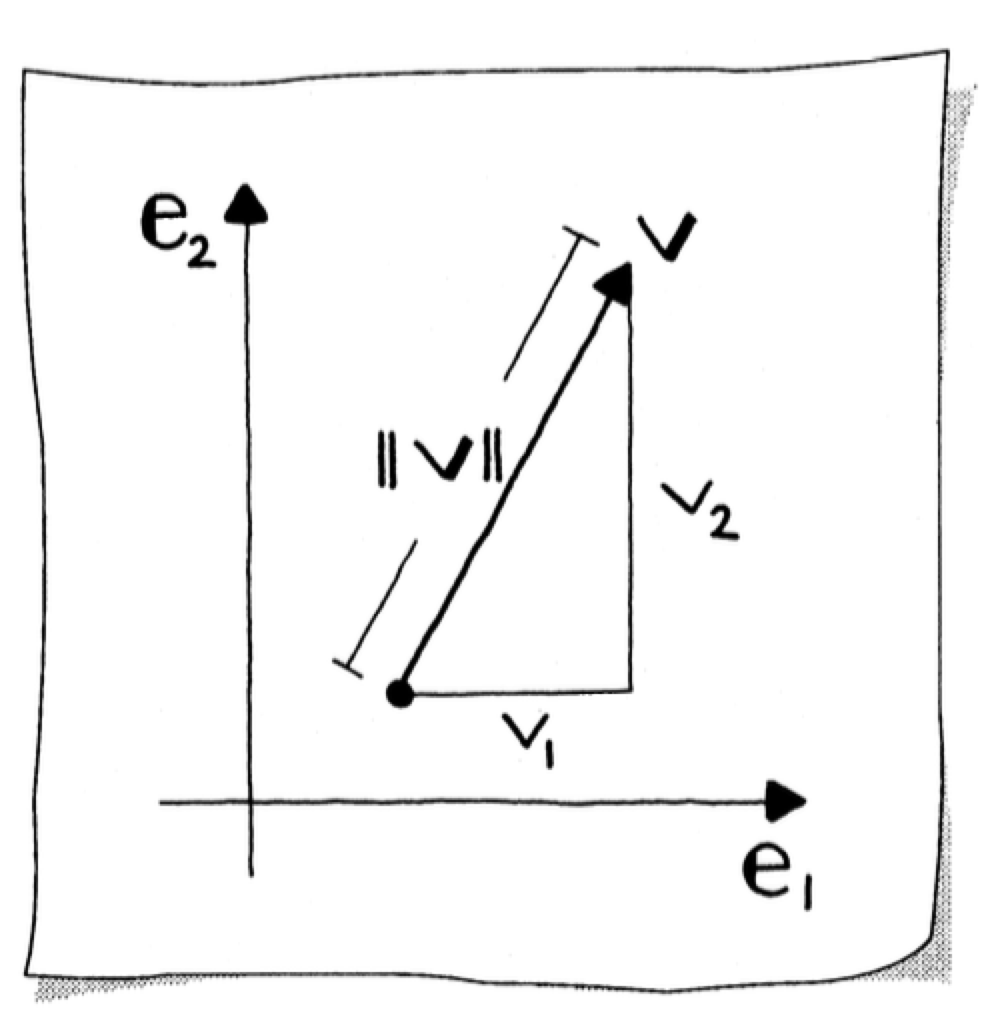
This is also called the Euclidean norm. For a point $\mathbf{X} = \lbrack x, y \rbrack^T$, the distance from the origin $\lbrack 0, 0 \rbrack^T$ is $\sqrt{x^2 + y^2}$, and we define this to be the length of the vector, written $\lvert\mathbf{X}\rvert$ or $\lVert\mathbf{X}\rVert$.
Examples:
- If $\mathbf{X} = \lbrack 3, 4 \rbrack^T$, then $\lvert\mathbf{X}\rvert = \sqrt{3^2 + 4^2} = 5$
- The standard basis vector $\mathbf{e}_1 = \lbrack 1, 0 \rbrack^T$ has $\lvert\mathbf{e}_1\rvert = 1$
- The zero vector has $\lvert\mathbf{0}\rvert = \sqrt{0^2 + 0^2} = 0$
Vector Length is Always Non-Negative
Since the square root is always considered positive or zero, the length of a vector is never negative. In fact, $\lvert\mathbf{X}\rvert$ is strictly positive unless $\mathbf{X} = \mathbf{0}$.
Scalar Multiplication and Length
For any scalar $r$:
\[\lvert r\mathbf{X}\rvert = \left\lvert \begin{bmatrix} rx \\ ry \end{bmatrix} \right\rvert = \sqrt{(rx)^2 + (ry)^2} = \sqrt{r^2 x^2 + r^2 y^2} = \lvert r\rvert \sqrt{x^2 + y^2} = \lvert r\rvert\lvert\mathbf{X}\rvert\]
Thus, the length of a scalar multiple of a vector equals the length of the vector multiplied by the absolute value of the scalar. For example, $\lvert -5\mathbf{X}\rvert = \lvert -5\rvert\lvert\mathbf{X}\rvert = 5\lvert\mathbf{X}\rvert$.
julia> v = [2, 2]
2-element Vector{Int64}:
 2
 2

julia> sqrt(v[1]^2 + v[2]^2)
2.8284271247461903

julia> norm(v)
2.8284271247461903

julia> norm(v) == sqrt(v[1]^2 + v[2]^2)
true
Unit Vectors
A unit vector (or normalized vector) $\mathbf{w}$ has length equal to one:
\[\lVert\mathbf{w}\rVert = 1\]
Normalizing a Vector
If $\mathbf{X} \neq \mathbf{0}$, we may scale by the reciprocal $1/\lvert\mathbf{X}\rvert$ to get a unit vector:
\[\mathbf{w} = \frac{\mathbf{v}}{\lVert\mathbf{v}\rVert}\]
This vector lies along the ray from $\mathbf{0}$ to $\mathbf{X}$ and has length 1 since:
\[\left\lvert \frac{1}{\lvert\mathbf{X}\rvert} \mathbf{X} \right\rvert = \left\lvert \frac{1}{\lvert\mathbf{X}\rvert} \right\rvert \lvert\mathbf{X}\rvert = \frac{1}{\lvert\mathbf{X}\rvert} \lvert\mathbf{X}\rvert = 1\]
Each component of $\mathbf{v}$ is divided by the scalar value $\lVert\mathbf{v}\rVert$. This scalar is always non-negative, meaning zero or greater. You must check the value before dividing to ensure it exceeds your zero divide tolerance—the absolute value of the smallest number by which you can divide confidently.
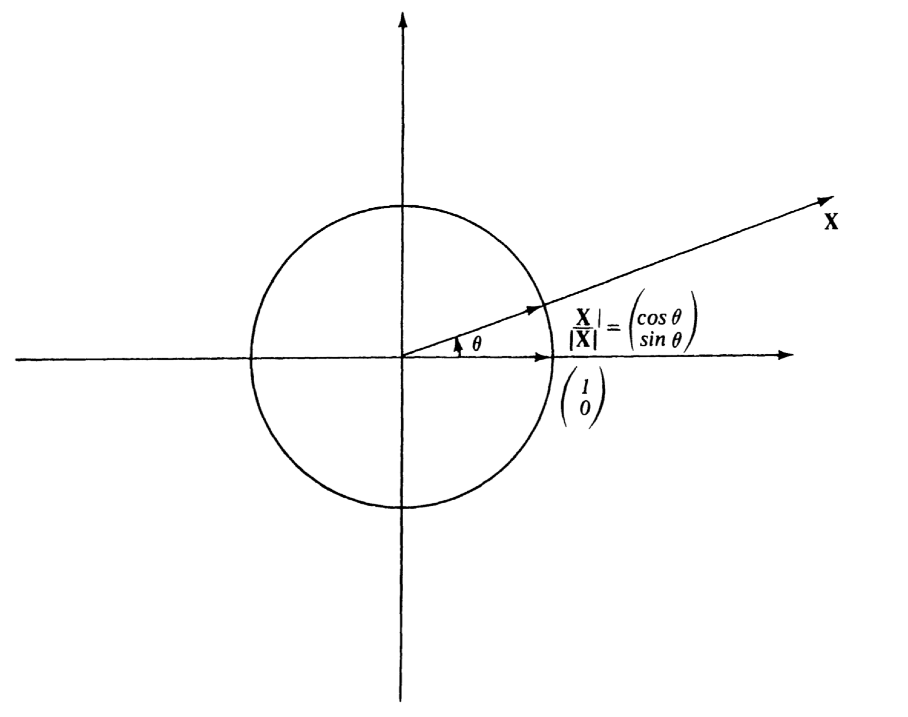
The vectors of length 1 are represented by points on the unit circle in the coordinate plane. There are infinitely many unit vectors; drawing them all emanating from the origin produces a circle of radius one.
julia> w = v / norm(v)
2-element Vector{Float64}:
 0.7071067811865475
 0.7071067811865475

julia> norm(w)
0.9999999999999999

julia> round(norm(w))
1.0
Polar Form of a Vector
Any vector on the unit circle may be described by its angle $\theta$ from the positive $x$-axis. We call $\theta$ the polar angle of the vector. The unit vector can be written using trigonometric functions as:
\[\begin{bmatrix} \cos\theta \\ \sin\theta \end{bmatrix}\]
If $\mathbf{X}$ is any non-zero vector, we have:
\[\mathbf{X} = \lvert\mathbf{X}\rvert \left(\frac{1}{\lvert\mathbf{X}\rvert} \mathbf{X}\right) = \lvert\mathbf{X}\rvert \begin{bmatrix} \cos\theta \\ \sin\theta \end{bmatrix} = \begin{bmatrix} \lvert\mathbf{X}\rvert \cos\theta \\ \lvert\mathbf{X}\rvert \sin\theta \end{bmatrix}\]
This representation as a positive scalar multiple of a unit vector is called the polar form of the vector, since we have written the coordinates in the form of polar coordinates.
Examples:
- If $\mathbf{X} = \lbrack 3, 0 \rbrack^T$, we have $\mathbf{X} = 3\mathbf{e}_1$, where $\mathbf{e}_1 = \lbrack \cos(0), \sin(0) \rbrack^T$
- If $\mathbf{X} = \lbrack 1, 1 \rbrack^T$, then $\mathbf{X} = \sqrt{2}\lbrack 1/\sqrt{2}, 1/\sqrt{2} \rbrack^T = \sqrt{2}\lbrack \cos\theta, \sin\theta \rbrack^T$, where $\theta = 45^\circ = \pi/4$
function polar_unit(y::Vector)
    [(y[1]/norm(y)), (y[2]/norm(y))]
end

julia> y = [1, 1]
julia> z = polar_unit(y)
2-element Vector{Float64}:
 0.7071067811865475
 0.7071067811865475

julia> norm(y) * z
2-element Vector{Float64}:
 1.0
 1.0

julia> round(acosd(z[1]))
45.0
Dot Product (Algebraic Definition)
Given two vectors $\mathbf{v}$ and $\mathbf{w}$, we might ask:
- Are they the same vector?
- Are they perpendicular to each other?
- What angle do they form?
The dot product is the tool to resolve these questions.
Motivation from the Pythagorean Theorem
Consider two perpendicular vectors $\mathbf{v}$ and $\mathbf{w}$. By the Pythagorean theorem:
\[\lVert\mathbf{v} - \mathbf{w}\rVert^2 = \lVert\mathbf{v}\rVert^2 + \lVert\mathbf{w}\rVert^2\]
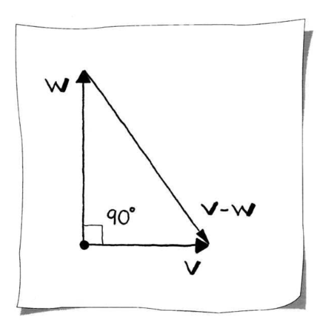
Writing the components explicitly:
\[(v_1 - w_1)^2 + (v_2 - w_2)^2 = (v_1^2 + v_2^2) + (w_1^2 + w_2^2)\]
Expanding and simplifying:
\[(v_1^2 - 2v_1w_1 + w_1^2) + (v_2^2 - 2v_2w_2 + w_2^2) - (v_1^2 + v_2^2) - (w_1^2 + w_2^2) = 0\]
This reduces to:
\[v_1w_1 + v_2w_2 = 0\]
We find that perpendicular vectors have the property that the sum of the products of their components is zero.
Definition
For two arbitrary vectors $\mathbf{v}$ and $\mathbf{w}$, we define the dot product as:
\[s = \mathbf{v} \cdot \mathbf{w} = v_1w_1 + v_2w_2\]
The dot product returns a scalar $s$, which is why it is also called a scalar product. Mathematicians also call it an inner product.
Constructing Perpendicular Vectors
A vector $\mathbf{w}$ perpendicular to a given vector $\mathbf{v}$ can be formed by switching components and negating one:
\[\mathbf{w} = \begin{bmatrix} -v_2 \\ v_1 \end{bmatrix}\]
Then $\mathbf{v} \cdot \mathbf{w} = v_1(-v_2) + v_2v_1 = 0$.
Dot Product and Vector Length
The dot product is a fundamental operation in linear algebra that connects algebraic computations with geometric concepts like angles and perpendicularity. The dot product of a vector with itself gives the square of its length:
\[\mathbf{X} \cdot \mathbf{X} = \begin{bmatrix} x \\ y \end{bmatrix} \cdot \begin{bmatrix} x \\ y \end{bmatrix} = x^2 + y^2 = \lvert\mathbf{X}\rvert^2\]
Therefore, the length of any vector is the square root of the dot product with itself:
\[\lVert\mathbf{X}\rVert = \sqrt{\mathbf{X} \cdot \mathbf{X}}\]
We have $\mathbf{X} \cdot \mathbf{X} \geq 0$ for all $\mathbf{X}$, with equality if and only if $\mathbf{X} = \mathbf{0}$.
Dot Product Properties
The dot product has the following algebraic properties for vectors $\mathbf{u}, \mathbf{v}, \mathbf{w} \in \mathbb{R}^2$:
| Property | Formula |
|---|---|
| Symmetric (Commutative) | $\mathbf{u} \cdot \mathbf{v} = \mathbf{v} \cdot \mathbf{u}$ |
| Homogeneous | $\mathbf{v} \cdot (s\mathbf{w}) = s(\mathbf{v} \cdot \mathbf{w})$ |
| Distributive | $(\mathbf{v} + \mathbf{w}) \cdot \mathbf{u} = \mathbf{v} \cdot \mathbf{u} + \mathbf{w} \cdot \mathbf{u}$ |
| Positive Definite | $\mathbf{v} \cdot \mathbf{v} > 0$ if $\mathbf{v} \neq \mathbf{0}$, and $\mathbf{v} \cdot \mathbf{v} = 0$ if $\mathbf{v} = \mathbf{0}$ |
Geometric Interpretation and the Law of Cosines
The dot product has a powerful geometric interpretation connecting it to the angle between vectors.
Derivation via the Law of Cosines
From trigonometry, the height $h$ of a triangle can be expressed as:
\[h = \lVert\mathbf{w}\rVert \sin(\theta)\]
Squaring and using the identity $\sin^2(\theta) + \cos^2(\theta) = 1$:
\[h^2 = \lVert\mathbf{w}\rVert^2 (1 - \cos^2(\theta))\]
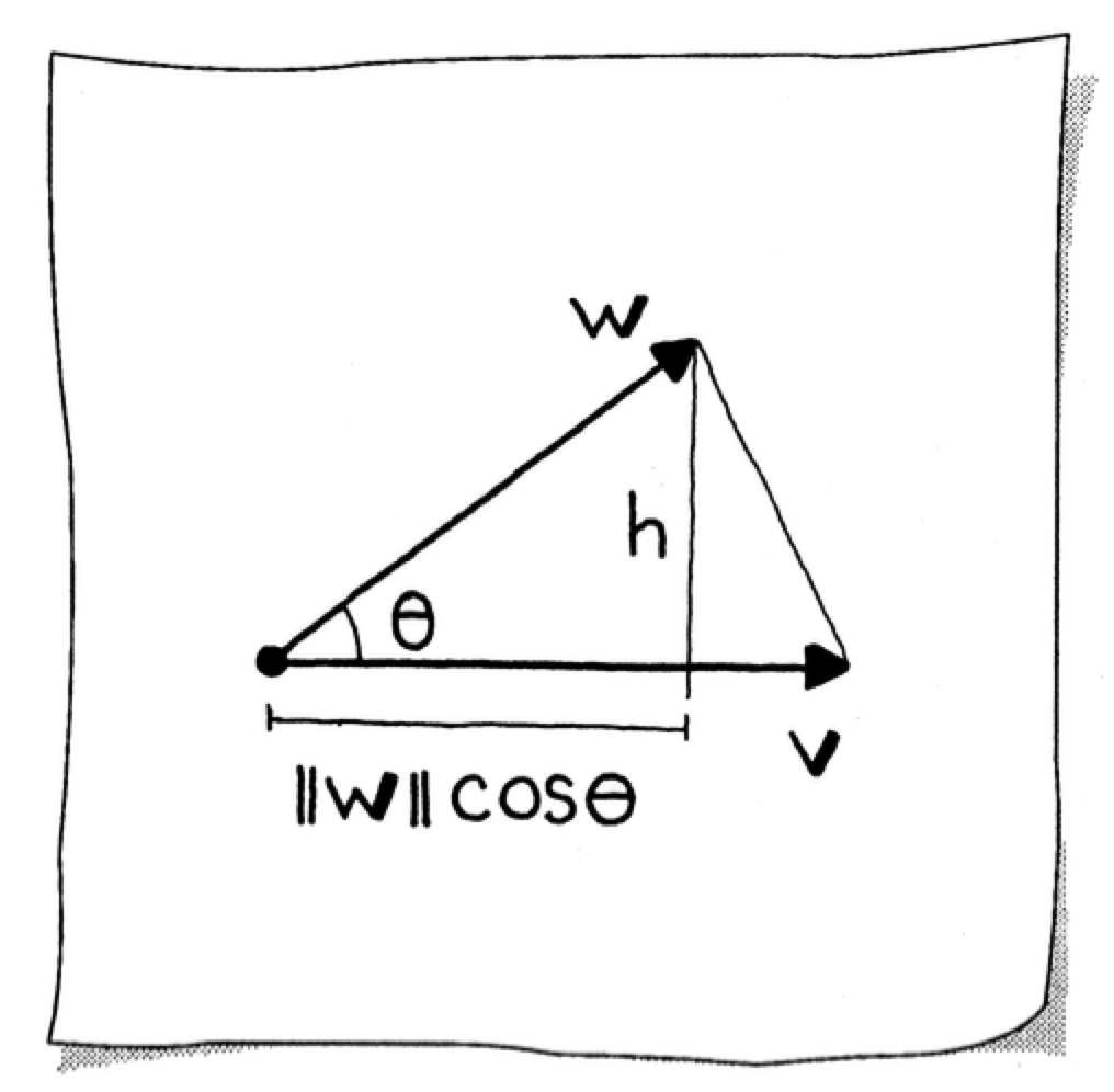
We can also express $h^2$ using the other right triangle and the Pythagorean theorem:
\[h^2 = \lVert\mathbf{v} - \mathbf{w}\rVert^2 - (\lVert\mathbf{v}\rVert - \lVert\mathbf{w}\rVert\cos\theta)^2\]
Equating and simplifying yields the Law of Cosines:
\[\lVert\mathbf{v} - \mathbf{w}\rVert^2 = \lVert\mathbf{v}\rVert^2 + \lVert\mathbf{w}\rVert^2 - 2\lVert\mathbf{v}\rVert\lVert\mathbf{w}\rVert\cos\theta\]
This generalizes the Pythagorean theorem for triangles with an opposing angle different from $90^\circ$.
Geometric Formula for the Dot Product
We can also write $\lVert\mathbf{v} - \mathbf{w}\rVert^2$ using the dot product:
\[\begin{aligned} \lVert\mathbf{v} - \mathbf{w}\rVert^2 &= (\mathbf{v} - \mathbf{w}) \cdot (\mathbf{v} - \mathbf{w}) \\ &= \lVert\mathbf{v}\rVert^2 - 2\mathbf{v} \cdot \mathbf{w} + \lVert\mathbf{w}\rVert^2 \end{aligned}\]
Equating the two expressions, we find the geometric formula for the dot product:
\[\mathbf{v} \cdot \mathbf{w} = \lVert\mathbf{v}\rVert\lVert\mathbf{w}\rVert\cos\theta\]
Dot Product and Cosines
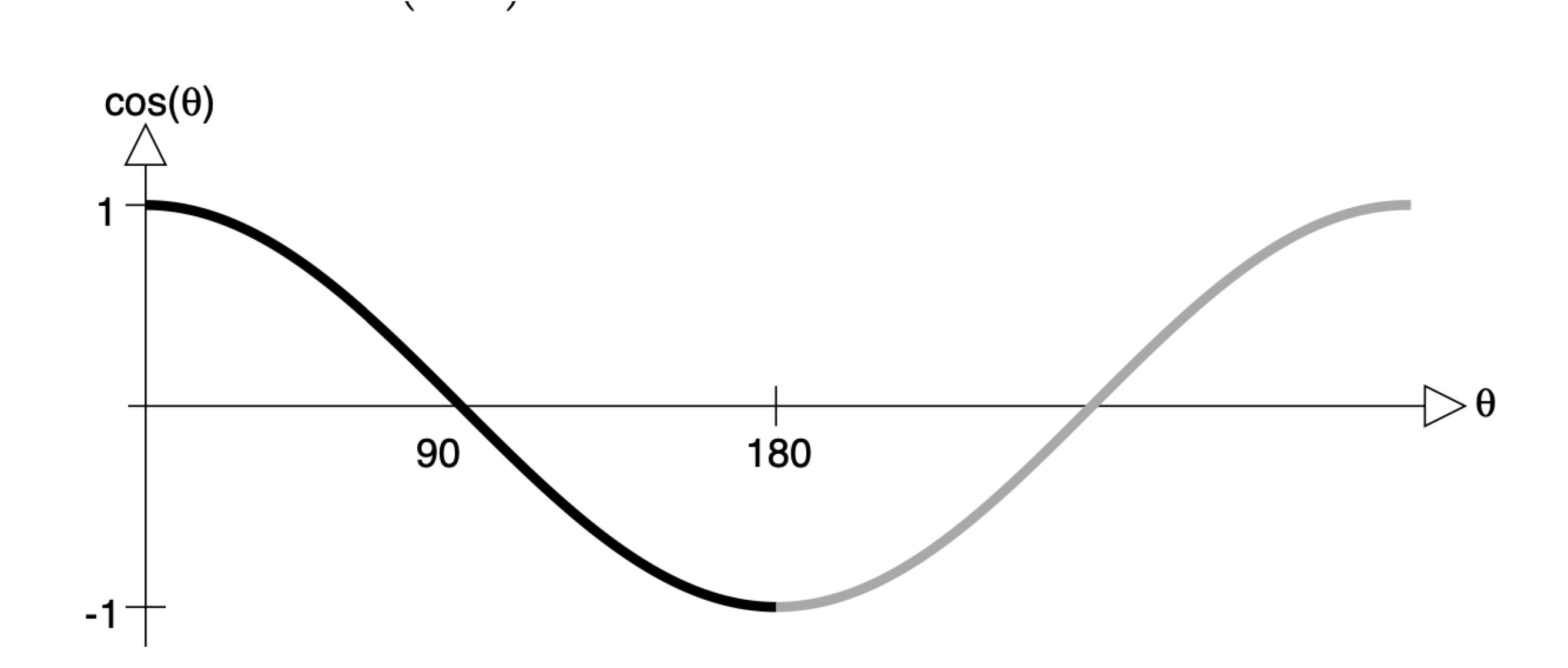
Rearranging the geometric formula, the cosine of the angle between two vectors is:
\[\cos\theta = \frac{\mathbf{v} \cdot \mathbf{w}}{\lVert\mathbf{v}\rVert\lVert\mathbf{w}\rVert}\]
Special Cases
Perpendicular vectors: The dot product is zero, giving $\cos(90^\circ) = 0$.
Parallel vectors: If $\mathbf{v} = k\mathbf{w}$ (same or opposite direction):
\[\cos\theta = \frac{k\mathbf{w} \cdot \mathbf{w}}{\lvert k\rvert\lVert\mathbf{w}\rVert\lVert\mathbf{w}\rVert} = \frac{k\lVert\mathbf{w}\rVert^2}{\lvert k\rvert\lVert\mathbf{w}\rVert^2} = \pm 1\]
This corresponds to $\theta = 0^\circ$ (same direction) or $\theta = 180^\circ$ (opposite direction).
Angle Classification
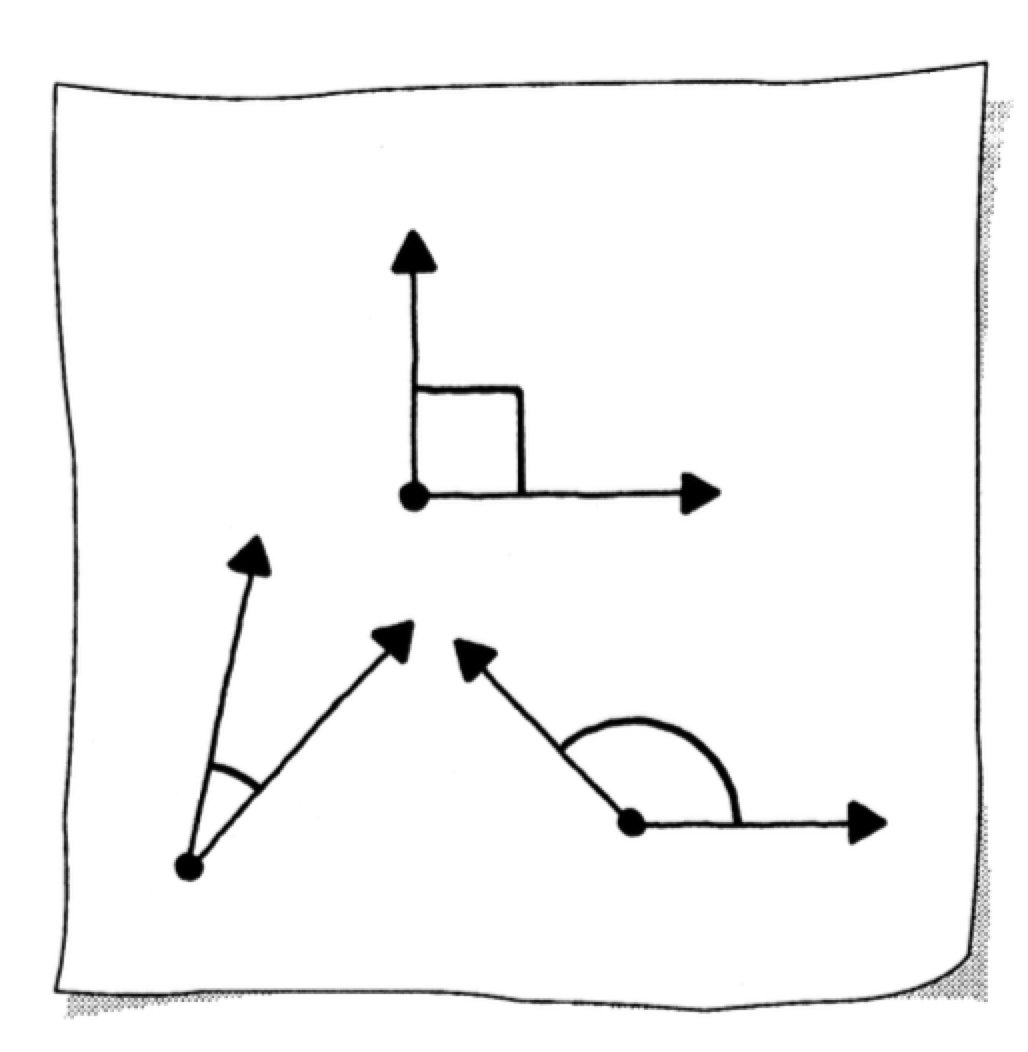
The cosine values range between $\pm 1$, corresponding to angles between $0^\circ$ and $180^\circ$. Three types of angles can be formed:
| Angle Type | Condition | Dot Product |
|---|---|---|
| Right | $\cos(\theta) = 0$ | $\mathbf{v} \cdot \mathbf{w} = 0$ |
| Acute | $\cos(\theta) > 0$ | $\mathbf{v} \cdot \mathbf{w} > 0$ |
| Obtuse | $\cos(\theta) < 0$ | $\mathbf{v} \cdot \mathbf{w} < 0$ |
Computing the Angle
To calculate the actual angle $\theta$, use the arccosine function:
\[s = \frac{\mathbf{v} \cdot \mathbf{w}}{\lVert\mathbf{v}\rVert\lVert\mathbf{w}\rVert}, \quad \theta = \arccos(s)\]
function vector_angle_cos(p::Point, q::Point)
    s = dot(p, q) / (norm(p) * norm(q))
end

julia> v = Point(2, 1)
julia> w = Point(-1, 0)
julia> s = vector_angle_cos(v, w)
-0.8944271909999159

julia> acos(s)
2.677945044588987

julia> acosd(s)  # In degrees
153.434948822922
Caution: In some math libraries, if $s > 1$ or $s < -1$, an error occurs returning NaN. Due to floating-point roundoff, an intended value of $s = 1.0$ might become $s = 1.0000001$. Always check that $s$ is within $\lbrack -1, 1 \rbrack$ before computing arccosine. In many applications (such as comparing angles), the cosine itself suffices without computing the actual angle.
Orthogonal Vectors
Two vectors are orthogonal (perpendicular) if and only if their dot product is zero:
\[\mathbf{X} \cdot \mathbf{U} = 0 \iff \mathbf{X} \perp \mathbf{U}\]
Geometric Proof
When do we have $\mathbf{X} \cdot \mathbf{U} = xu + yv = 0$ for nonzero vectors?
One possibility is that one vector lies along the $x$-axis and the other along the $y$-axis—clearly perpendicular.
If $\mathbf{X}$ does not lie on either axis, then $x \neq 0$ and $y \neq 0$. The slope of the line from the origin through $\lbrack x, y \rbrack^T$ is $y/x$. Since $xu + yv = 0$, we have $yv = -xu$. If $u \neq 0$, then:
\[-1 = \frac{yv}{ux} = \frac{y}{x} \cdot \frac{v}{u}\]
Thus, the slope $v/u$ of the line to $\mathbf{U}$ is the negative reciprocal of $y/x$, meaning the lines are perpendicular. This relationship between perpendicular lines and negative reciprocal slopes connects to the discussion of line equations in 02 Lines.
function is_orthogonal(p::Point, q::Point)
    dot(p, q) == 0
end

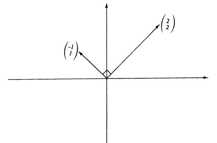
julia> u = Point(-1, 1)
julia> x = Point(2, 2)
julia> is_orthogonal(x, u)
true
Orthogonality and Line Equations
For any vector $\lbrack x, y \rbrack^T$, the vector $\lbrack -y, x \rbrack^T$ is perpendicular to it. This leads to an important connection with line equations (see 02 Lines for the implicit form of a line).
The line with equation:
\[ax + by = 0\]
can be described in two equivalent ways:
As a set of perpendicular vectors: The set of all vectors $\mathbf{X} = \lbrack x, y \rbrack^T$ perpendicular to the normal vector $\mathbf{n} = \lbrack a, b \rbrack^T$
As a direction vector: The line along the vector $\lbrack -b, a \rbrack^T$ (since this vector is perpendicular to $\lbrack a, b \rbrack^T$)
This connects the algebraic concept of orthogonality to the geometric representation of lines through the origin, which is foundational for understanding projections and transformations covered in later sections.
Summary
| Concept | Formula |
|---|---|
| Vector length | $\lVert\mathbf{v}\rVert = \sqrt{v_1^2 + v_2^2}$ |
| Unit vector | $\hat{\mathbf{v}} = \mathbf{v}/\lVert\mathbf{v}\rVert$ |
| Polar form | $\mathbf{X} = \lvert\mathbf{X}\rvert\lbrack\cos\theta, \sin\theta\rbrack^T$ |
| Dot product (algebraic) | $\mathbf{v} \cdot \mathbf{w} = v_1w_1 + v_2w_2$ |
| Dot product (geometric) | $\mathbf{v} \cdot \mathbf{w} = \lVert\mathbf{v}\rVert\lVert\mathbf{w}\rVert\cos\theta$ |
| Angle between vectors | $\cos\theta = \frac{\mathbf{v} \cdot \mathbf{w}}{\lVert\mathbf{v}\rVert\lVert\mathbf{w}\rVert}$ |
| Orthogonality condition | $\mathbf{v} \perp \mathbf{w} \iff \mathbf{v} \cdot \mathbf{w} = 0$ |
| Perpendicular vector | $\mathbf{w} = \lbrack -v_2, v_1 \rbrack^T$ is perpendicular to $\mathbf{v} = \lbrack v_1, v_2 \rbrack^T$ |